JSC Internals

0x00 Overview

This post is a summary of what I learned while solving the JSC wargame. Since I had already studied V8, diving into JSC felt like a fresh experience. In this post, I’ll walk through JSC’s execution pipeline, starting from LLInt, moving through the baseline JIT, and exploring DFG.

0x01 JSC Internals

I’ll be exploring JSC’s architecture and its JIT tiers, but rather than tracing every function in detail, I’ll focus on the key aspects and differences between each JIT tier. If you’re interested in a full deep dive into JSC by tracing every function, check out JavaScriptCore Internals Part I. The following sections provide a concise summary of Parts 1 to 5 from that resource.

JSC shell

The JSC shell provides a REPL(Repeat-Eval-Print-Loop) environment, allowing the engine to parse and execute JavaScript interactively. Thanks to the JSC shell, you can test JSC independently without having to build the entire WebKit project. When launching the shell, it sets up the WTF(Web Template Framework), initializes WebKit codebase functions, and handles VM object memory allocation.

Runtime Setup

At runtime, the JSC engine focuses on three key objectives:

1. Lexing and parsing the source code
2. Generating bytecode from the parsed AST
3. Executing the generated bytecode

AST

The AST is constructed by processing the raw source code through lexing and parsing, which generates tokens and organizes them into a structured tree. During this process, ECMA spec validation is performed to detect syntax and semantic errors in the provided JavaScript script.

ByteCode

Before converting the generated AST into bytecode, it’s worth noting that WebKit has previously updated its bytecode format. I recommend reading the Webkit post for background on these changes.

Once the AST is built, bytecode isn’t generated immediately. Instead, an unlinked CodeBlock is created, and unlinked bytecode is populated within it. As the AST is traversed, opcodes, exception handlers, and try-catch nodes are identified and written into the unlinked bytecode. Only after this unlinked CodeBlock is fully constructed can the bytecode be executed or linked. This linking process iterates over the unlinked instructions stored in the CodeBlock, updating metadata tables based on opcodes. JSC provides specific debug options for each JIT tier, allowing us to observe its internal execution behavior. As an example, I’ll demonstrate one such case. When running JSC with a debug option enabled, you can inspect the generated bytecode via stdout, as shown below:

$ cat  test.js
let x = 10 + 20;
let y = x

$ ./jsc --dumpGeneratedBytecodes=true test.js

Bytecode generated from parsing test.js:

<global>#AodHI4:[0x7fe26eac8000->0x7fe2aeea8068, NoneGlobal, 57]: 12 instructions (0 16-bit instructions, 0 32-bit instructions, 6 instructions with metadata); 169 bytes (112 metadata bytes); 1 parameter(s); 10 callee register(s); 6 variable(s); scope at loc4

[   0] enter
[   1] get_scope          loc4
[   3] mov                loc5, loc4
[   6] check_traps
[   7] mov                loc6, Undefined(const0)
[  10] resolve_scope      loc7, loc4, 0, GlobalProperty, 0
[  17] put_to_scope       loc7, 0, Int32: 30(const1), 1048576<DoNotThrowIfNotFound|GlobalProperty|Initialization>, 0, 0
[  25] resolve_scope      loc7, loc4, 1, GlobalProperty, 0
[  32] resolve_scope      loc8, loc4, 0, GlobalProperty, 0
[  39] get_from_scope     loc9, loc8, 0, 2048<ThrowIfNotFound|GlobalProperty|NotInitialization>, 0, 0
[  47] put_to_scope       loc7, 1, loc9, 1048576<DoNotThrowIfNotFound|GlobalProperty|Initialization>, 0, 0
[  55] end                loc6

Identifiers:
  id0 = x
  id1 = y

Constants:
   k0 = Undefined
   k1 = Int32: 30: in source as integer

LLInt (Low Level Interpreter)

LLInt is an interpreter built using JIT’s calling convention. JSC starts by executing code in LLInt, and once the code is proven hot, it tiers up to a higher JIT level. At its core, LLInt iterates over bytecode, executing each instruction and then moving to the next. During execution, it maintains profiling information and counters that track execution frequency. These two parameters help optimize the code, enabling tiered JIT compilation through OSR(On-Stack Replacement).

LLInt is generated using OfflineASM, which has both advantages and drawbacks. However, its two key features are:

1. Portable assembly: allowing it to be adapted across different architectures
2. Macro constructs, simplifying complex low-level code generation

Fast Path/Slow Path

A key aspect of LLInt is the concept of fast and slow paths. LLInt is designed to generate fast code with low latency whenever possible. However, when generating bytecode, LLInt needs to determine the type of operands to select the correct execution path.

For example, consider the following JavaScript code:

let x = 10;
let y = {a : "Ten"};
let z = x+y;

In this code, if the types of x and y are different, LLInt will no longer be able to perform the addition. As a result, LLInt will follow the slow path, where it invokes C++ code to handle the operand type mismatch case and perform the necessary type checks or conversions.

Tiering Up

When bytecode has been executed more than a certain number of times in LLInt, it is profiled as warm code, and if deemed hot, it can be tiered up to a higher JIT tier. LLInt primarily determines whether a function or loop is “hot” or if the code should tier up based on execution counts. LLInt’s execution counters are governed by various rules, with thresholds varying depending on the situation. The threshold for transitioning from LLInt to Baseline uses a static threshold of 500 executions. However, for other optimizing tiers that use dynamic thresholds, the tiering-up threshold is calculated based on various factors and dynamic values. These dynamic thresholds allow the JIT compiler to adapt and optimize more effectively depending on the actual execution profile and runtime behavior of the code.

Baseline JIT

Baseline JIT is a template JIT that generates specific machine code for bytecode operations. It provides a significant performance boost over LLInt for two main reasons:

• Removal of interpreter dispatch: This eliminates the overhead of calling the interpreter for each bytecode operation.
• Comprehensive support for polymorphic inline caching: This optimizes frequently accessed methods or properties by caching their results, improving lookup speeds.

When LLInt tiers up to Baseline JIT, it performs a quick check to determine whether the CodeBlock needs JIT compilation. If compilation is necessary, a new thread is created to handle OSR. Using MacroAssemblers, the bytecode is compiled into machine code, specifically targeting the instructions in the bytecode stream. During this process, machine code for stack management routines is also generated, which is crucial for the correct handling of stack frames in Baseline JIT compiled code.

Fast Path/Slow Path

As observed when reviewing LLInt, there are two execution paths. In Baseline JIT, additional optimizations are performed for opcodes that implement both fast and slow paths. While iterating through the opcodes implemented on the slow path, machine code is generated, and if necessary, the jump table is modified.

Linking

Once the CodeBlock is successfully compiled, the next step is to link the machine code to OSR from LLInt to the Baseline JIT optimized code. This process involves replacing the current execution path with the newly generated machine code, allowing for more efficient execution as the code transitions to a higher-performance JIT tier.

execution

Once OSR is complete in the JITed code, the engine will search for the OSR entry. Once found, the engine will jump from LLInt to the JITed code, allowing execution to continue at the optimized level.

The purpose of Profiling Tiers
1. We just want to know if the bad thing ever happened: Profiling tiers help identify when performance bottlenecks or issues arise, such as type mismatches or slow execution paths, allowing the system to respond appropriately.
2. Profiling Tiers aim to compile hot functions sooner: By profiling execution, the JIT compilers can quickly identify frequently executed (hot) functions and prioritize their compilation to optimized machine code, improving overall performance.

Tier up

The process of tiering up from Baseline JIT to DFG (Data-Flow Graph) is similar to the transition from LLInt to Baseline JIT. To tier up from Baseline JIT to DFG, the static execution count threshold must be surpassed. This threshold is set to 1000 executions. Once this threshold is reached, DFG compilation is triggered. If the compilation is successful, the engine obtains the OSR entry for the target address, enabling the transition to the DFG-compiled code.

DFG (Data Flow Graph)

DFG (Data Flow Graph), being an optimizing compiler, introduces various vulnerabilities like type confusion, OOB access, and information leaks in the JIT source code. These vulnerabilities arise due to the complexity of dynamic optimizations and the manipulation of data flow during the compilation process.

Here is an image summarizing the DFG pipeline along with the previous steps:

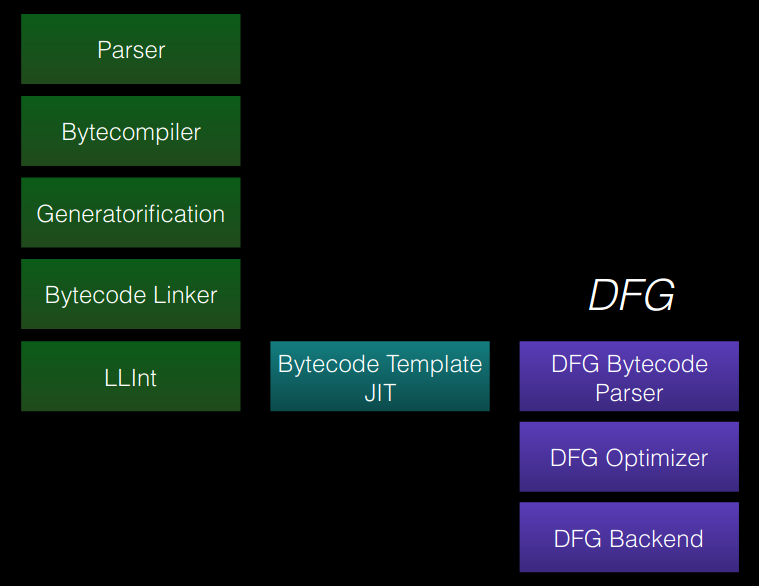dfg pipeline stage(https://zon8.re/posts/jsc-part3-the-dfg-jit-graph-building)

Before tiering up from Baseline JIT to DFG via OSR, DFG performs the following key tasks:

1. Parsing the bytecodes in the CodeBlock to a graph
2. Optimizing the graph
3. Generating machine code from the optimized graph

Bytecode parsing

The first step of DFG compilation is parsing the bytecode to create a graph. During this process, the jump targets in the bytecode are collected. For each jump target, the process iterates through the bytecode to create blocks, nodes, and edges, which form an unoptimized graph. This graph is represented as DFG IR.

DFG IR

This IR (Intermediate Representation) is used in both DFG and FTL tiers. When compiling with DFG, the generated DFG graph block includes a Header, Block Head, Block Body, Nodes, Edges, Tail, and Footer.

The role of each element is as follows:

• Graph Header: Memory address of the codeblock, optimization status, graph type, type, reference count, and function arguments.
• Block Head: Execution info of the BasicBlock, variable states, and the flow relationships between blocks.
• Block Body
  • Node: Represents individual opcodes with NodeIndex, NodeType, NodeFlags, Operands, and NodeOrigin.
  • Edge: Refers to the nodes that a particular node depends on.
• Block Tail: Restores variable states and OSR Exit information at the end of the block.
• Graph Footer: Contains GC values, watchpoints, and a list of structures associated with the CodeBlock.

Function Inlining

Function inlining is an optimization technique used to reduce the overhead of frequently called functions. To perform function inlining, it’s necessary to determine if the function is hot, if there are no exceptions or complex control flows within the function, and if it has low polymorphism and predictable behavior.

DFG Optimisation

The goal of DFG optimization is to remove as many type checks as possible to enable faster compilation. DFG performs key optimizations through static analysis of the generated graph. There are three main static analyses in DFG that have a significant impact on optimization decisions:

1. Prediction Propagation: Predicts all types.
2. Abstract Interpreter: Finds redundant OSR speculation, reducing OSR checks.
3. Clobberize: Gathers aliasing information about DFG operations.

Clobberize
Clobberize is the alias analysis that the DFG uses to describe what parts of the program’s state an instruction could read and write. This allows us to see additional dependency edges between instructions beyond just the ones expressed as data flow. Clobberize has many clients in both the DFG and FTL.

The steps of DFG optimization are as follows:

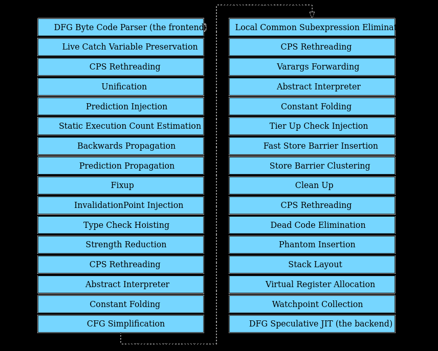dfg optimisation(https://zon8.re/posts/jsc-part3-the-dfg-jit-graph-building)

The DFG pipeline consists of 30 optimization steps, with 25 of them being unique optimizations. Let’s go over the role of each optimization.

Live Catch Variable Preservation

Live Catch Variable Preservation preserves live variables in a “catch” block by flushing them to the stack from the “try” block, ensuring that variables are maintained during an OSR exit.

CPS Rethreading

CPS Rethreading transforms the existing LoadStore type graph into a ThreadedCPS form, making it more suitable for data flow analysis, register allocation, and code generation.

Unification

Unification integrates the VariableAccessData of Phi nodes and their child nodes, creating a “lifetime range splitting” view of the variables.

Prediction Injection

Prediction Injection uses profiling data to inject predicted types of variables into IR nodes, enabling more efficient subsequent optimization and code generation.

Static Execution Count Estimation

The Static Execution Count Estimation phase estimates execution counts and execution weights for branch and switch nodes based on static information. It also calculates dominators for various blocks, which is helpful for the CFG Simplification phase.

Backwards Propagation

Backwards Propagation evaluates and merges node flags from the last block to the first, updating the flags to provide additional information on how the computed value of a node is used.

Prediction Propagation

Prediction Propagation propagates predictions gathered from heap load sites and slow path executions to generate a predicted type for each node in the graph. After this phase, full type information is available for all nodes in the graph.

Fixup

Fixup is a phase that corrects inefficient portions of the graph based on predictions.

Invalidation Point Injection

Invalidation Point Injection inserts InvalidationPoint nodes at the beginning of any CodeOrigin. These points check for triggered watchpoints and can lead to an OSR Exit from the optimized code.

Type Check Hoisting

Type check hoisting is the process of promoting redundant structure and array checks to variable assignments when the structure’s transition watchpoint set is valid, or the variable’s live range does not affect the structure.

Strength Reduction

Strength Reduction is a phase that performs optimizations that don’t depend on CFA or CSE. It mainly handles simple transformations like constant folding.

Control Flow Analysis

Control Flow Analysis combines type predictions and type guards to create type proofs and propagate them globally within the code block.

Constant Folding

onstant Folding eliminates unnecessary operations by substituting constants.

CFG Simplification

CFG simplification simplifies control flow by merging or removing unnecessary blocks, potentially changing the graph significantly. Dead code is eliminated, and the graph format is reset.

Local Common Subexpression Elimination

The Local Common Subexpression Elimination phase identifies and removes redundant nodes, optimizing the graph by redirecting edges to other nodes.

Variable Arguments Forwarding

The Variable Arguments Forwarding phase eliminates allocations of Arguments objects and optimizes the graph by forwarding values from candidate nodes.

Tier Up Check Injection

Tier Up Check Injection phase inserts tier-up checks for code blocks with FTL enabled. The checks are added at the head of loops and before function returns to optimize performance.

Fast Store Barrier Insertion

The Fast Store Barrier Insertion phase inserts store barriers to ensure memory ordering, avoiding barriers on newly allocated objects.

Store Barrier Clustering

The Store Barrier Clustering phase clusters barriers that can be executed in any order and optimizes their placement.

Cleanup

Cleanup phase removes unnecessary nodes like empty Check and Phantom nodes.

Dead Code Elimination

Dead Code Elimination phase removes unused or unnecessary nodes.

Phantom Insertion

Phantom Insertion phase inserts Phantom nodes to preserve children of nodes killed during graph optimization based on bytecode liveness.

Stack Layout

Stack Layout phase remaps used local variables to optimize the stack layout and eliminate any holes.

Virtual Register Allocation

Virtual Register Allocation phase assigns spill slots(i.e the virtual register) to nodes to determine where values will be stored in the call frame.

Watchpoint Collection

Watchpoint Collection phase collects watchpoints for DFG nodes that meet specific conditions in the graph.